
Argo temperature and salinity measurements during the period 2005 to 2010 are used to estimate GOIs such as GOHC (Global Ocean Heat Content) and GSSL (Global Steric Sea Level).
Global Ocean Indicators
![]()
![]()
![]()
Indicator from the MyOcean in-situ Thematic Assembly Center (TAC)
by K. von Schuckmann*(1) and P.-Y. Le Traon (2)
*Corresponding author : Karina von Schuckmann
(1) CNRS/LOCEAN Paris, hosted by Ifremer-LOS Brest, France
(2) IFREMER - LOS, Brest, France
PRODUCT USER MANUAL ( PUM ) : HERE
QUALITY INFORMATION DOCUMENT ( QUID) : HERE
The product can be downloaded via a ftp link. The “FTP download” allows to download an entire dataset directly from the FTP server at the supply center.
ACCESS TO THE PRODUCT : HERE
If you do not have MyOcean login, see : http://www.myocean.eu/web/27-registration.php
Context
Globally integrated time series based on in situ measurements which are named here Global Ocean Indicators (GOIs, von Schuckmann and Le Traon, 2011) are a useful benchmark and an important diagnostic to study changes of the Earth’s climate system from which the global ocean provides the largest contribution (Hansen et al., 2005; Levitus et al., 2005, Cazenave and Llovel, 2010, Hansen et al., 2011; Church et al., 2011). GOIs presented here include Global Ocean Heat Content (GOHC) and Global Steric Sea Level (GSSL) calculated from the global observing system Argo (Roemmich et al., 2009; http://www.argo.ucsd.edu/). Estimations of GOHC contribute to the calculation of the Earth’s energy imbalance which is the amount of energy to which the climate system has not yet responded to (e.g. Hansen et al., 2005, Trenberth et al., 2009, Church et al., 2011, Hansen et al., 2011). Also the calculation of the global sea level budget is an important aspect for research of climate related changes. The largest contribution to global mean sea level come from ocean volume changes (steric changes) and ocean mass changes, i.e. the melting of glaciers and ice caps (e.g. Leuliette and Miller, 2009, Cazenave and Llovel, 2010, Church et al., 2010, Church et al., 2011). Accurate estimations of GSSL are hence important to quantify this budget.
Description of the method
Argo temperature and salinity measurements during the period 2005 to 2010 are used to estimate GOIs such as GOHC and GSSL. We developed a method based on a simple box averaging scheme using a weighted mean (von Schuckmann and Le Traon, 2011). Uncertainties due to data processing methods and choice of climatology are estimated. This method is easy to implement and run and can be used to set up a routine monitoring of the global ocean.
An Argo climatology (ACLIM hereinafter, 2004–2009, von Schuckmann et al., 2009) is first interpolated on every profile position in order to fill gappy profiles at depth of each temperature and salinity profile. This procedure is necessary to calculate depth-integrated quantities. At every profile position, heat storage changes are calculated as the integral from 10 to 1500 m depth of ρcpT’(z)dz where T’ is the anomaly relative to ACLIM of Argo temperature data provided from the MyOcean in-situ Thematic Assembly Center (MyOcean product name: INS-CORIOLIS-GLO-TS-DT_OA_OBS) and using the reference density ρ = 1030 kg.m-3 and the specific heat capacity cp = 3980 J/kg°C. Similarly, steric sea level is calculated as the integral from 10 to 1500m depth ΔD=∫pα(S,T,P)dp-∫pα(35,0,P)dP, where α is the specific volume which is equal to the inverse of density [Gilson et al., 1998]. Density is calculated from temperature and salinity data provided from the MyOcean in-situ Thematic Assembly Center (MyOcean product name: INS-CORIOLIS-GLO-TS-DT_OA_OBS). Then, anomalies of steric sea level are calculated at every profile position using ACLIM.
To estimate GOIs from the irregularly distributed profiles, the global ocean is divided into boxes of 5° latitude, 10° longitude and 3 month size. This provides a sufficient number of observations per box. To remove spurious data, measurements which depart from the mean at more than 3 times the standard deviation are excluded. The variance information to build this criterion is derived from ACLIM. This procedure excludes about 1% of data from our analysis. Only data points which are located over bathymetry deeper than 1000m depth are then kept. Boxes containing less than 10 measurements are considered as a measurement gap. Finally, the parameters are averaged globally, weighted by their surface area.
First results
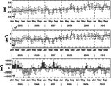
The results for GOHC and GSSL are shown in Figure 1. Over the six year time period, trends of GOHC and GSSL are 0.54±0.1Wm−2 and 0.75±0.15mmyr−1, respectively. These results are valid under the assumption that no systematic errors remain in the observing system. This indicator will be updated every year from reprocessed, delayed mode data. It is of utmost importance to associate precise error bars to these estimations which is a non trivial exercise. The error bar which is composed of the measurement error, the data processing procedure and climatology uncertainties is marked in Figure 1 (see von Schuckmann and Le Traon, 2011 for more details on the error calculation). More work will be done on the error estimation. These efforts include comparisons to other data sets to improve the error estimation.

References
- Cazenave, A., and W. Llovel, 2010: Contemporary Sea Level Rise, Annu. Rev. Mar. Sci., 2, 145–73.
- Church, J.A., P.L. Woodworth, T. Aarup, S. Wilson, 2010: Understanding sea-level rise and variability, John Wiley & Sons, London.
- Church, J.A., N.J. White, L.F. Konikow, C.M. Domingues, J.G. Cogley, E. Rignot, J.M. Gregory, M.R. van den Broeke, A.J. Monaghan, and I. Velicogna, 2011: Revisiting the Earth’s sea level and energy budgets from 1961 to 2008, Geophysical Research Letters, 38, L18601, doi:10.1029/2011GL048794.
- Gilson, J., D. Roemmich, B. Cornuelle, and L.-L. Fu, 1998: Relationship of TOPEX/Poseidon altimetric height to steric height and circulation in the North Pacific, J. Geophys. Res., 103, 27,947–27,965.
- Hansen, J., L. Nazarenko, and R. Ruedy, and M. Sato, and J. Willis, and A. Del Genio, and D. Koch, and A. Lacis, and K. Lo, and S. Menon, and T. Novakov, and J. Perlwitz, and G. Russell, and G.A. Schmidt, and N. Tausnev, 2005: Earth's Energy Imbalance: Confirmation and Implications, Science, 308, 1431-1435, doi:10.1126/science.1110252
- Hansen, J., M. Sato, P. Kharecha, and K. von Schuckmann, 2011: Earth's energy imbalance and implications, Atmos. Chem. Phys. Discuss., 11, 27031-27105, www.atmos-chem-phys- discuss.net/11/27031/2011/, accepted.
- Leuliette, E.W., and L. Miller, 2009: Closing the sea level rise budget with altimetry, Argo, and GRACE, Geophysical Research Letters, 36, L04608, doi:10.1029/2008GL036010.
- Levitus, S., J. Antonov, and T. Boyer, 2005: Warming of the World Ocean, 1955-2003, Geophys.Res.Lett., 32, doi:10.1029/2004GL021892
- Roemmich, D., and A.S. Team: Argo, 2009: The challenge of continuing 10 years of progress. Oceanography, 20, 26-35.
- Trenberth, K.E., J.T. Fasullo, and J. Kiehl, 2009: Earth’s global energy budget, BAMS, American Meteorological Society,doiI:10.1175/2008BAMS2634.1.
- von Schuckmann, K. , F. Gaillard and P.-Y. Le Traon, 2009: Global hydrographic variability patterns during 2003-2008, Journal of Geophysical Research, in press.
- von Schuckmann, K., and P.-Y. Le Traon, 2011: How well can we derive Global Ocean Indicators from Argo data? Ocean Sci., 7, 783–791, www.ocean-sci.net/7/783/2011/, doi:10.5194/os-7-783-2011.